Managing Data Collection and Analysis Assignment Sample

Best data sources:

• Local customer data: Talking to people who visit and shop in town centres in Birmingham.
• Market research reports: Available surveys or findings about what people drink.
• Social media: Looking at social media and reading online reviews to examine what hot drinks customers are talking about near your place (LI, LARIMO and LEONIDOU, 2022).

Three data collection methods:

1. Distribute questionnaires to shoppers that will help you discover their favourite type of hot drink.
2. Check how many purchases are made at the set places and log what people order.
3. Organise small groups for discussions and use the results to better understand what people prefer.

B. Analysis of collected data

i. Pie chart

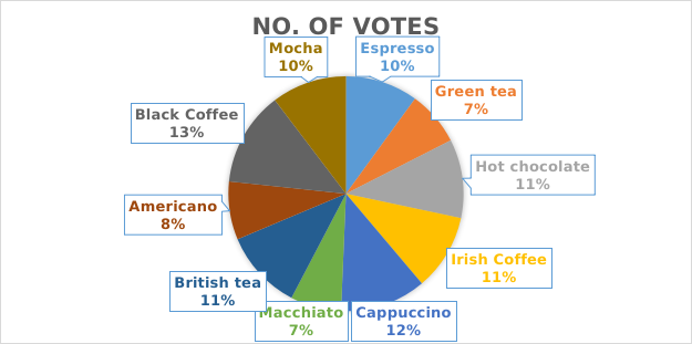
ii Most popular hot drink and relative frequency

Most popular hot drink - Black Coffee with 78 votes.

Relative frequency

= (Number of votes for Black Coffee) / (Total votes)

= 78 / 600 = 0.13 or 13%

C. Linear Programming problem for crop planting

Variables:

• Let x = hectares of Barley
• Let y = hectares of Wheat

i. Formulation:

Objective function (maximize profit):

Maximize ;Z=100x+150y

Subject to constraints:

1. Budget constraint (cost):

50x + 20y ≤ 500

2. Labour constraint (man-days):

1x+2y ≤ 40

3. Land constraint (total land):

x+y ≤ 40

4. Non-negativity constraints:

x≥0,y≥0

ii. Plotting the linear programming graph

Land constraint = X + Y â‰¤ 40

Labor constraint = X + 2Y â‰¤ 40

Cost constraint = 50X + 20Y â‰¤ 500

Labour and cost constraints intersect at points

50X + 20Y = 500

-10(X + 2Y = 40)

= (40X = 100)

= X = 2.5

If X=2.5, the value of Y = 18.75

Graphical representation:

iii) Optimal hectares to grow for maximum profit

Find the corner points of the feasible region by solving the intersections:

1. Intersection of budget and labour constraints:
Solve:

50x+20y=500 ------Eq 1

x+2y=40---------Eq 2

From Eq 2:

x=40−2y

Substitute into Eq 1:

50(40−2y)+20y=500

2000−100y+20y=500

2000−80y=500

80y=1500

y=18.75

Then,

x=40−2(18.75) =2.5

Check profit at (2.5, 18.75):

Z =100(2.5)+150(18.75)

=250+2812.5

=3062.5

Checking profit at (0, 20):

Z =100(0)+150(20)

=3000

Checking profit at (10, 0):

Z =100(10)+150(0)

=1000

Thus, the best possible solution keeping in mind all the constraints is (2.5, 18.75) 

Get free assignment examples!

QUESTION 2

A. Difference between simple mean and geometric mean

Simple Mean (Arithmetic Mean):

The amount you receive by dividing the total of your values by the number of values. This importance lies in using this average for data that are additive and can be arranged in any order.

Geometric Mean:

The nth root of the product of all values. Data growth rates or ratios are good examples, especially when values show sharp and endless increases (Vogel, 2020). It shows the average rate that you would receive every period to have the same outcome.

Geometric Mean = (1.03 * 1.12 * 1.15 * 1.16 * 1.14 * 0.91 * 1.20 * 1.09 * 1.07) ^(1/9)

=1.0934

Deducting 1 for getting the geometric mean:

1.0934-1 = 0.0934 or 9.34%

B. Definition and characteristics of Linear Regression

To model and understand the connection between a dependent variable and one or more independent variables, linear regression fits a line to data points observed in a study.

In simple linear regression, you express the connection between X and Y in the following way:

Y = β₀ + β₁X + ε

Three important characteristics of linear regression:

• The connection between the independent and dependent variables follows a straight, reliable pattern.
• Observations are independent of each other.
• When data is homoscedastic, the variance in the residuals stays the same as values of the independent variable increase or decrease.

C. Plotting simple linear regression with regression equation and coefficient of determination

D. Interpretation of regression equation and coefficient of determination

The regression equation derived from the data is Y=65.25+1.76X, where Y represents sales revenue and X indicates expenses for sales promotion which are shown in thousands of pounds. That's why the expected revenue with free promotion is £65,250. Sales promotion spending of an extra £1,000 usually results in a boost of £1,760 to the sales revenue. It is possible to see that putting money into promotions helped increase Nescafé's sales revenue. Additionally, the coefficient of determination, R². This shows that sales promotion costs account for 85% of the difference in sales revenue from one year to another. This strong R² value indicates an obvious linear relationship between promotion expenses and sales revenue.

QUESTION 3

A (i) Calculation of NPV:

Discount rate = 9%

Business A:

Net present value for Business A: 33686.61 

Business B:

Net present value for Business B: 34680.27 

ii) Recommendation:

The analysis of NPVs determines that Business B has the higher value, with 34,680.27, so Samuelson should go with this option. It is foreseen that, over the next five years, Business B is likely to bring better results while accounting for the value of time. Because Business B's NPV is higher, it shows greater cash inflows that lead to successful and enduring growth (Shou, 2022). According to the findings, Samuelson will get the most value from Business B and it will be more likely to succeed in the long run. As a result, from a money standpoint, it is wise to buy Business B.

B. Probability and modal group analysis:

B (i). Probability of individual distance to the workplace is “0.1 to 2.50”:

= Resident living between 0.1 to 2.50 / Total residents

= (0+1+6+37+29+31+7) / 390

= 111/390 = 0.2846 or 28.46% 

B (ii). Probability of an individual spending over £280:

= (Amount spent over 280) / Total residents

= (46+13) / 390

= (59/390) = 0.1513 or 15.13%

B (iii). Probability of an individual spending “£151 - £190” and the distance to the workplace is “2.52 - 6.0” miles:

= 55 / 390 = 0.1410 or 14.10%

C. Modal group as per category of Amount Spent, £:

Modal group = 241-280 (frequency= 111 residents)

QUESTION 4

A) Arithmetic Mean (μ) = 72

S.D (σ)= 6

Top 25% means cut-off score is at 75th percentile

75^th percentile = 0.674 (z-score)

Z-score formula: (X-μ) / Ïƒ

Putting values into formula:

0.674= (x-72)/6

Shuffling formula to find test scores:

Test score (X): (0.674*6) + 72

                        : 4.044+72 = 76.044 or 76 (approx.)

Minimum marks desired to pass interview are 76. 

B)

B (i). In the chart, the uniform distribution is seen since the probability density function does not change between a and b. Here, the probability density function is provided as:

f(x) = 1/(b-a)

Minimum value (a) = 80

Maximum value (b) = 160

Using formula, we get

Probability density of distribution is = f(x) = 1 / (160-80)

= 1/80 or 0.0125 

B (ii). Mean and standard deviation:

Mean (μ)= (a+b)/2 = (80 + 160) / 2 = 120 grams

Standard deviation (σ) = √((b-a) ^2)/12

= √ ((160-80) ^2)/12    = √ 533

    = 23.094 grams

 Answer b (ii)

Mean = 120 grams

Standard deviation 23.094 grams.

B (iii). Probability of a candidate taking vegetables:

Total Width of range = (120 - 95) = 25 grams

Total range value = (160-80) = 80 grams

Formula for Probability

= (Total width of range) / (Total range)

Probability = 25/ 80 = 0.3125 or 31.25%

Answer. Candidates take vegetable between 95 to 120 grams are 31.25%. 

C. Normal Distribution:

• A pattern of data that is continuous, symmetric and shaped like a bell, determined by a mean (μ) and standard deviation (σ) (Jaya Sreevalsan-Nair, 2022).
• The position of the center in a distribution is determined by the mean and the spread is controlled by the standard deviation.
• Most data is found close to the mean and probabilities fall off evenly on either side of it.
• All the points under the curve add up to 1 which shows the total probability.

Standard Normal Distribution:

• A normal distribution that is set with a mean of 0 and a standard deviation of 1.
• All probabilities and z-scores are based on this reference.
• To change any normal distribution into a standard normal distribution, use the formula to standardize the data.

Z = (X-μ)/ Ïƒ

• It holds a bell curve and is the same on both sides of zero.

REFERENCES

Andrade, C. (2021). Z Scores, Standard Scores, and Composite Test Scores Explained. Indian Journal of Psychological Medicine, 43(6), pp.555-557. doi: https://doi.org/10.1177/02537176211046525.

Jaya Sreevalsan-Nair (2022). Normal Distribution. Encyclopedia of earth sciences series/Encyclopedia of earth sciences, pp.1-4. doi: https://doi.org/10.1007/978-3-030-26050-7_228-1.

LI, F., LARIMO, J. and LEONIDOU, L.C. (2022). Social Media in Marketing research: Theoretical bases, Methodological aspects, and Thematic Focus. Psychology & Marketing, 40(1), pp.124-145. doi:https://doi.org/10.1002/mar.21746.

Rotondi, A., Pedroni, P. and Pievatolo, A. (2022). Probability, Statistics and Simulation. Unitext. Springer International Publishing. doi: https://doi.org/10.1007/978-3-031-09429-3.

Shou, T. (2022). A Literature Review on the Net Present Value (NPV) Valuation Method. [online] www.atlantis-press.com. doi: https://doi.org/10.2991/aebmr.k.220603.135.

Vogel, R.M. (2020). The geometric mean? Communications in Statistics - Theory and Methods, pp.1-13. doi: https://doi.org/10.1080/03610926.2020.1743313.

UPTO51%

Avail The Benefit Today!

To View this & another 50000+ free

Enter Email

Submit